
Article Outline
#(99%自分用メモ)RcmdrPlugin.KMggplot2にテーマ追加
(注意)OSはLinux。/home/(ユーザー名)/R/x86_64-pc-linux-gnu-library/(Rバージョン)にインストール。
関連記事:(99%自分用メモ)RcmdrPlugin.KMggplot2にメニュー追加
RcmdrPlugin.KMggplot2で定義している各boxの使い方はわかりやすい。plot-factorise.rを参考にするとグラフ作成しないメニューも作れそう。
- vbbox : 変数の選択
- lbbox : ラベルの入力(テキスト)
- rbbox : ラジオボタン(どれか一つ)
- cbbox : チェックボックス(選択するしない)
- tbbox : テーマ、色、フォントサイズ
(windowsならRtoolsが必要。)
- Rcmdr : 2.7.2
- RcmdrPlugin.KMggplot2 : 0.2.6
- ggplot2 : 3.3.5
- ggmosaic : 0.3.3
ggthemes内のテーマを選べるようにしてある。が、個人的には使わないと思う。
使いそうなテーマ(theme_classicの凡例の位置を変えただけ)を作って追加した。
ただ、追加、変更箇所(ファイル)はメニューを追加したときより多くなる。
追加、変更箇所(ファイル)
- plot-aaa.r : checkTheme に書式をまねて、
theme_classicR,theme_classicLを追加
こんなふうに
        else if (index == "theme_classicL") {
        theme <- "RcmdrPlugin.KMggplot2::theme_classicL"
      } else if (index == "theme_classicR") {
        theme <- "RcmdrPlugin.KMggplot2::theme_classicR"
guiparts-toolbox.r :
theme <<- variableListBoxにtheme_classicR,theme_classicLを登録DESCRIPTION : Collate に
'theme_classicL.r''theme_classicR.r'を追加NAMESPACE :
export(theme_classicL)export(theme_classicR)を追加
さらに、Rフォルダー内のrファイルの中には "legend.position = \"right\"" と記述しているものがあるのでその箇所をコメントアウトする必要がある。
(念の為、削除はしない)
検索してみると、該当するrファイルは、
plot-gkm.r、plot-gscat.r、plot-gline.r、plot-gscatmat.r、plot-ghist.r、plot-gdiscbar.r、
plot-gcont.r、plot-gpie.r
グラフ作成の手順
テーマにtheme_classicを選択。「プレビュ」を押してプロットを確認。
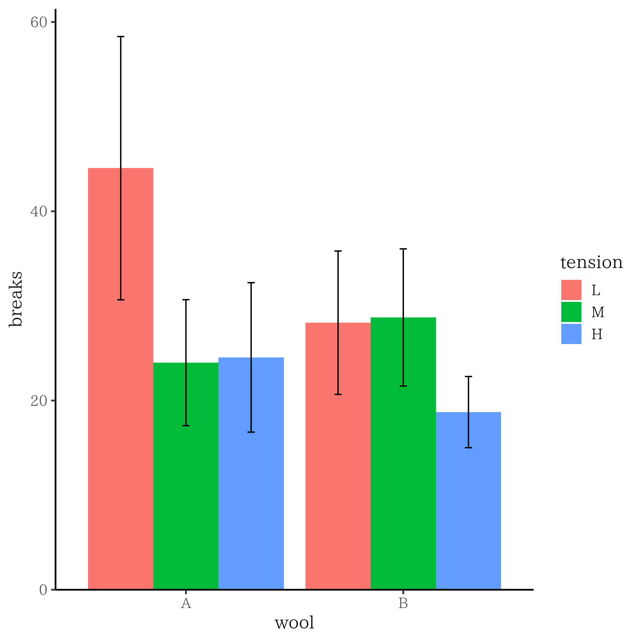
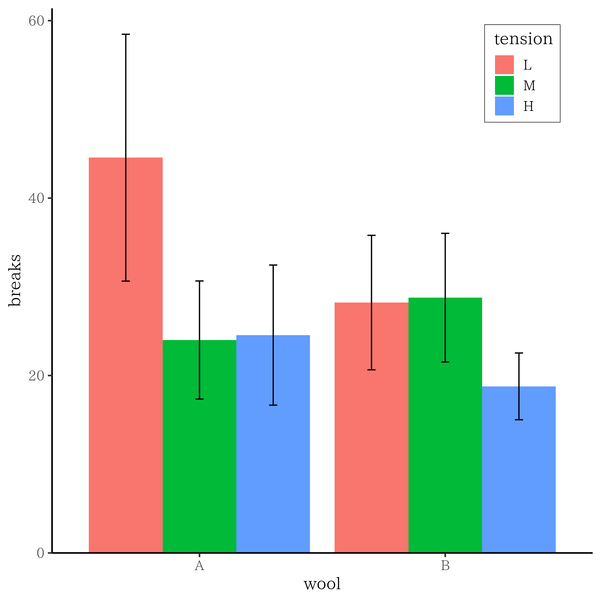
グラフ右上があいているので、 theme_classicRを選択。「プレビュ」を押してプロットを確認。「OK」を押して決定。
なお、棒グラフやヒストグラムをプロットする際、グラフの範囲とx軸の隙間はないほうが好みなので該当する.rファイルの
scale_y_continuous にexpand = expansion(mult = c(0, 0.05))と記述した。
作成したテーマ
この他にもグリッド線が必要な場合のために3つ(凡例:右外、右上、左上)登録しています。
theme_classicR.r
theme_classicの凡例の位置をグラフ内の右上にした。
theme_classicR <- function(base_size = 11, base_family = "",
                          base_line_size = base_size / 22,
                          base_rect_size = base_size / 22) {
  theme_bw(
    base_size = base_size,
    base_family = base_family,
    base_line_size = base_line_size,
    base_rect_size = base_rect_size
  ) %+replace%
    theme(
      # no background and no grid
      panel.border     = element_blank(),
      panel.grid.major = element_blank(),
      panel.grid.minor = element_blank(),
      # show axes
      axis.line      = element_line(colour = "black", size = rel(1)),
      # match legend key to panel.background
#      legend.key       = element_blank(),
# legend:left
 legend.position=c(0.8,0.97),
 legend.justification=c(0,1),
 legend.background = element_rect(fill = "white", colour = "black",size =0.2),
 legend.margin=margin(5,6,5,8),
      # simple, black and white strips
      strip.background = element_rect(fill = "white", colour = "black", size = rel(2)),
      # NB: size is 1 but clipped, it looks like the 0.5 of the axes
      complete = TRUE
    )
}
theme_classicL.r
theme_classicの凡例の位置をグラフ内の左上にした。
theme_classicL <- function(base_size = 11, base_family = "",
                          base_line_size = base_size / 22,
                          base_rect_size = base_size / 22) {
  theme_bw(
    base_size = base_size,
    base_family = base_family,
    base_line_size = base_line_size,
    base_rect_size = base_rect_size
  ) %+replace%
    theme(
      # no background and no grid
      panel.border     = element_blank(),
      panel.grid.major = element_blank(),
      panel.grid.minor = element_blank(),
      # show axes
      axis.line      = element_line(colour = "black", size = rel(1)),
      # match legend key to panel.background
#      legend.key       = element_blank(),
# legend:left
 legend.position=c(0.03,0.97),
 legend.justification=c(0,1),
 legend.background = element_rect(fill = "white", colour = "black",size =0.2),
  legend.margin=margin(5,6,5,8),
      # simple, black and white strips
      strip.background = element_rect(fill = "white", colour = "black", size = rel(2)),
      # NB: size is 1 but clipped, it looks like the 0.5 of the axes
      complete = TRUE
    )
}